Introduction

Neural network’s most basic unit is a neuron. The way neurons interact and work together is the main determinant of the limits of a neural network’s complexity and sophistication. Similar to neurons found in the human brain, once a neuron receives a signal it is capable of combining it through linear regression, transforming it, and producing a new signal that is then received by another neuron.

Neural networks are often seen in layers, with neurons in different levels interacting through the weighted attachments. Essentially, neurons in the same layers will receive the same inputs, and the outputs will be combined in the next layer’s neurons.

A neural network can be created using programming libraries or GUI applications. However, in this project we will be using calculus and Numpy to code a fully functional network from scratch using state of the art algorithms like HE initialization and ADAM optimization.

Architechting The Layers

Our goal is to create a function that can accept any vertex and transform it into vectorized neural layers.

For initializing the weights of W and b, we will be using the HE initialization method which was proven to be better than random initialization. Later on, we will use ADAM optimization so we are also initializing the hyperparameters (V & S) for that function now in order to reduce the reliance on extra for loop.


def initialize_he(layers_dims):
    V = {}
    S = {}
    parameters = {}
    L = len(layers_dims) - 1 
    for l in range(1, L + 1):
        parameters['W' + str(l)] = np.random.randn(layers_dims[l], layers_dims[l-1]) * np.sqrt(2 / layers_dims[l-1])
        V['dW'+str(l)] = np.zeros_like(parameters["W" + str(l)])
        S['dW'+str(l)] = np.zeros_like(parameters["W" + str(l)])
        parameters['b' + str(l)] = np.zeros((layers_dims[l], 1))
        V["db" + str(l)] = np.zeros_like(parameters["b" + str(l)])
        S["db" + str(l)] = np.zeros_like(parameters["b" + str(l)])
    return parameters,V,S

Forward Propagation

Forward propagation is the easiest part of neural network architecture. In order to propagate all of our training examples we will be using a matrix dot product. We need a function that accepts training examples, the initialized weight, and the type of the activation functions in which layers will be dropped in order to reduce overfitting.

First: we use matrix dot product to compute Z

\[X.W_1+b_1\] Where X is the input matrix and W are the first layer weights and b is the bias.

Then: We insert Z in the activation function to get A then repeat for all the layers

\[A.W_2+b_2\]

here is the complete code for forward propagation:

def forward(X,params,types,drop_layer):
  out = {}
  A=X
  L = len(types)

  for i in range(1,L+1):
    Z = np.dot(params['W'+str(i)],A)+ params['b'+str(i)]
    if types[i-1] == 'tanh':

      A = np.tanh(Z)
    elif types[i-1] == 'sigmoid':
      A = sigmoid(Z)

    elif types[i-1] =='relu':
      A =relu(Z)

    
    if i == drop_layer:
      A = dropout(A)
    

    out['Z'+str(i)] = Z
    out['A'+str(i)] = A

  
  out['A0']=X
  return out

Forward propagation dependencies

Because we are implementing a deep neural network in this example and we want our model to be non linear, the use of the Activation function is necessary. Without these functions, all the weights of different layers can be summed to a single layer and the sole purpose of the neural network is lost.

Our previous function relied on 3 activation functions (Tanh,Relu, sigmoid) and 1 drop function. Keep in mind that Tanh can be implemented natively in numpy. Later on, we will need the derivatives of these functions. In order to progress systematically. Let’s code all these functions now.

def sigmoid(Z):
    A = 1/(1+np.exp(-Z))
    
    return A 

def Dsigmoid(A):
  return A*(1-A)

def relu(Z):
  return np.maximum(Z,0)

def Drelu(z):
    return np.greater(z, 0).astype(int)

def Dtanh(A):
  return 1 - np.power(A, 2)


def compute_cost(AL, Y):
  
    
    m = Y.shape[1] # number of example
    logprobs = np.multiply(np.log(AL), Y) + np.multiply((1 - Y), np.log(1 - AL))
    cost = - np.sum(logprobs) / m
    cost = np.squeeze(cost)     # makes sure cost is the dimension we expect. 
                                # E.g., turns [[17]] into 17 
    
    
    return cost

Backward propagation

For backward propagation to be implemented, a function that takes into account X, Y, the predicted values of each example, and parameters (the weight and bias for each layer type) must be used. The function serves the purpose of calculating the derivatives of each variable. Relying heavily on calculus and using the helper function defined earlier. The result of this function is a dictionary that contains each derivative that will be used in updating the parameters.


def backward(X,Y,out, params,types):
  grads ={}
  L = str(len(types))
  Li = len(types)
  m = Y.shape[1]

  grads['dZ'+ L] = out['A'+ L ] - Y
  grads['dW'+L ] = (1/m)*(np.dot(grads['dZ'+L],out['A'+str(Li-1)].T))
  grads['db'+L] = (1/m)*(np.sum(grads['dZ'+ L],axis=1,keepdims=True))



  for i in range(Li-1,0,-1):
    
    if types[i-1] == 'tanh':
      grads['dZ'+ str(i)] = np.dot(params['W' +str(i+1)].T,grads['dZ' +str(i+1)])*(1-np.power(out['A'+ str(i)],2))

    if types[i-1] == 'relu':
      grads['dZ'+ str(i)] = np.dot(params['W' +str(i+1)].T,grads['dZ' +str(i+1)])*(Drelu(out['Z'+ str(i)]))
    

    
    grads['dW'+ str(i) ] = (1/m)*(np.dot(grads['dZ'+str(i)],out['A'+ str((i-1))].T))
    grads['db'+ str(i) ] = (1/m)*(np.sum(grads['dZ'+ str(i)],axis=1,keepdims=True))


  

  return grads

Updating the parameters

The ADAM (short for adaptive Moment Estimation ) optimization method uses Exponentially Moving Average combined with RMSProp Optimization. The main idea behind it is to average the weights across multiple examples in order to reduce the loss function fluctuations. It relies on 4 parameters, V and S which both have been initialized in a previous function, beta1(default = 0.9), and beta2(default = 0.999).

Here is a link from Cornell from Cornell University that explains the process very well.

Once you understand the algorithm, its application is fairly straightforward.


def update_with_Adam(params,grads,types,lr,V,S,beta1,beta2,t):
  L = len(types)
  V_C = {}
  S_C = {}


  for i in range(1,L+1):

    I = str(i)
    V['dW'+I] = beta1*V['dW'+I] + (1-beta1)*grads['dW'+I]
    V['db'+I] = beta1*V['db'+I] + (1-beta1)*grads['db'+I]

    V_C['dW'+I] = V['dW'+I]/(1-np.power(beta1,t))
    V_C['db'+I] = V['db'+I]/(1-np.power(beta1,t))

    S['dW'+I] = beta2*S['dW'+I] + (1-beta2)*np.power(grads['dW'+I],2)
    S['db'+I] = beta2*S['db'+I] + (1-beta2)*np.power(grads['db'+I],2)

    S_C['dW'+I] = S['dW'+I]/(1-np.power(beta2,t))
    S_C['db'+I] = S['db'+I]/(1-np.power(beta2,t))
    
    
    params['W'+I] = params['W'+I] - lr*(V_C['dW'+I]/np.sqrt(S_C['dW'+I]+1e-8)+1e-8)
    params['b'+I] = params['b'+I] - lr*(V_C['db'+I]/np.sqrt(S_C['db'+I]+1e-8)+1e-8)

  return params,V,S

Training with batches

To efficiently manage the increasing amounts of data it is necessary to split the data into smaller portions in order to train machine-learning models. There are many methods for dividing the training examples into batches. One example of these methods is stochastic. Stochastic trains one example at a time, training all the data at once, or using mini batches. The following function can be used to adjust the batch size for the required outcome. The drop layer position can also be specified here.

def batch_train_Adam(X,Y,P,types,iter,lr,drop_layer,batch_size,V,S,beta1,beta2):
  params = P
  m = X.shape[1]
  permutation = list(np.random.permutation(m))
  shuffled_X = X[:, permutation]
  shuffled_Y = Y[:, permutation].reshape((1,m))
  
  n_batches = m//batch_size
  t = 0

  for i in range(iter):
    permutation = list(np.random.permutation(m))
    shuffled_X = X[:, permutation]
    shuffled_Y = Y[:, permutation].reshape((1,m))

    for k in range(0,n_batches):
      X_batch = X[:,k*batch_size:(k+1)*batch_size]
      Y_batch = Y[:,k*batch_size:(k+1)*batch_size]

      out = forward(X_batch,params,types,drop_layer)
      grads = backward(X_batch,Y_batch,out, params,types)
      t= t+1
      params,V,S = update_with_Adam(params,grads,types,lr,V,S,beta1,beta2,t)
      

    if i%100==0:
      C = compute_cost(out['A'+str(len(types))],Y_batch)
      
      print('iteration :' +str(i))
      
      print(C)
  return params

Proof of Concept

This Neural Network Algorithm will be tested using a sklearn dataset that contains 300 examples and two labels.

We will be using a relatively small network (2 inner layers,10,5 nodes respectively) that matches the difficulty of this dataset. We won’t be using a dropout in this example as overfitting is currently not a concern.


def load_dataset():
    np.random.seed(1)
    train_X, train_Y = sklearn.datasets.make_circles(n_samples=300, noise=.05)
    np.random.seed(2)
    test_X, test_Y = sklearn.datasets.make_circles(n_samples=100, noise=.05)
    # Visualize the data
    plt.scatter(train_X[:, 0], train_X[:, 1], c=train_Y, s=40, cmap=plt.cm.Spectral);
    train_X = train_X.T
    train_Y = train_Y.reshape((1, train_Y.shape[0]))
    test_X = test_X.T
    test_Y = test_Y.reshape((1, test_Y.shape[0]))
    return train_X, train_Y, test_X, test_Y
  

train_X, train_Y, test_X, test_Y = load_dataset()

Although we did not write a time counter in our code, we can see the loss function dropped substantially during the first 200 iterations. However, it is expected to see some fluctuations since we are using batches.

params,V,S = initialize_he([2,10,5,1])
types = ['tanh','tanh','sigmoid']
new_params = batch_train_Adam(train_X,train_Y,params,types,2200,.08,'none',64,V,S,0.9,0.999)

## iteration :0
## 0.7005249085650023
## iteration :100
## 0.037945335057998575
## iteration :200
## 0.02884471735696274
## iteration :300
## 0.5007624771581856
## iteration :400
## 0.07187089059588332
## iteration :500
## 0.012795036396699249
## iteration :600
## 0.012769417802766785
## iteration :700
## 0.0183723889042458
## iteration :800
## 0.016292239382277515
## iteration :900
## 0.032524493623532644
## iteration :1000
## 0.013020023553337971
## iteration :1100
## 0.024472349000375076
## iteration :1200
## 0.007357900814325956
## iteration :1300
## 0.08110864477243597
## iteration :1400
## 0.0025365514742831338
## iteration :1500
## 0.00622510120565864
## iteration :1600
## 0.011314572610327197
## iteration :1700
## 0.0012947721943428556
## iteration :1800
## 0.0008670224949203275
## iteration :1900
## 0.0006849812105099117
## iteration :2000
## 0.022016205997497453
## iteration :2100
## 0.004208831618081026

Predictions

This model can be used to predict certain values with variable accuracies. It is seen in the graph below the differences between the test data and the model’s predictions’ results. The accuracy in this specific case is measured at 93% in a test data consisting of 100 samples, which shows that our implementation of a neural network using numpy is learning the patterns correctly. In order to improve the accuracy more nodes and layers should be used. Furthermore, it is worth noting that we only trained 300 samples where in a real situation the training data can be significantly bigger.

## 0.91

## Text(0.5, 1.0, 'Test Data')

## Text(0.5, 1.0, 'Prediction')

## Text(0.5, 0.98, 'Horizontally stacked subplots')

## <matplotlib.collections.PathCollection object at 0x000000006B406100>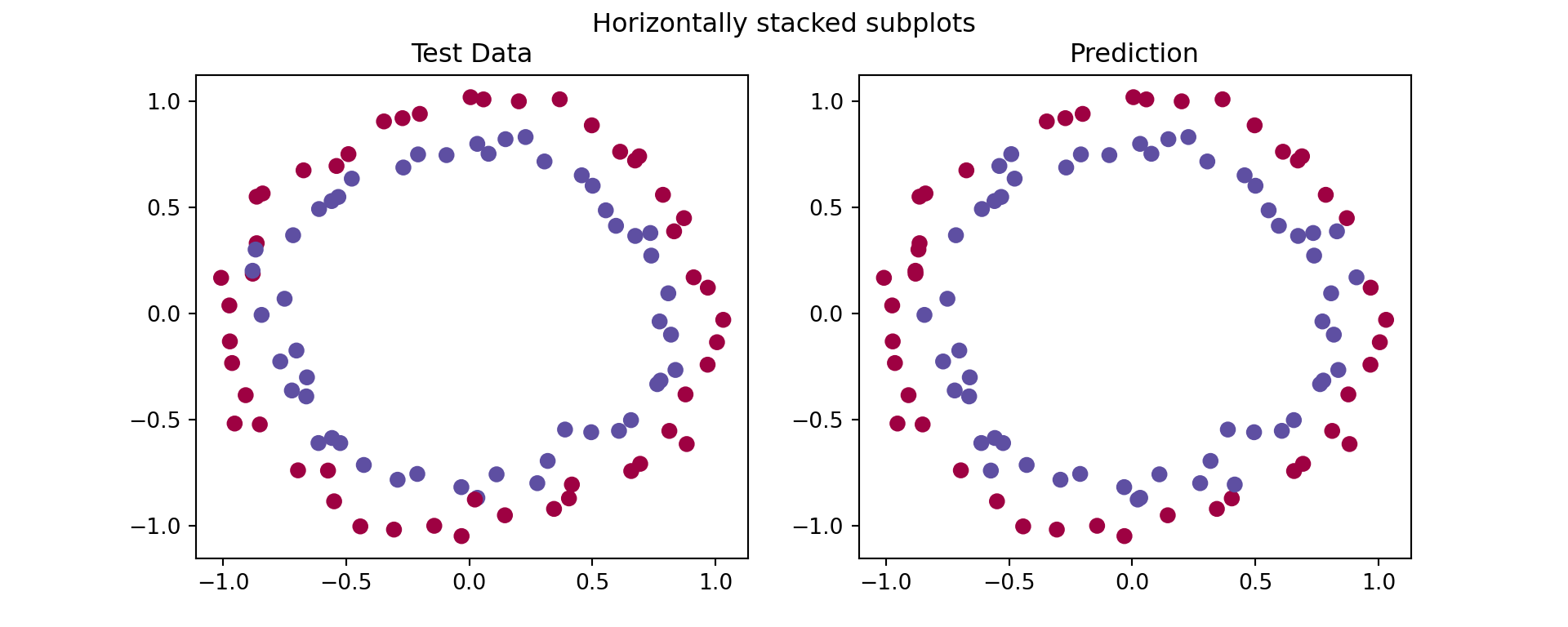

Conclusion

Although AI Libraries (Tensorflow-Pytorch) can perform neural networks algorithms with fewer lines of code, in order to fully understand the science behind these algorithms it’s recommended to do the math from scratch.